← All research|Also available in 中文
Adaptive Exposure Capping — why fixed drawdown limits fail in crypto regime shifts
Published: 2026-09-02
Simulated results — no real money. Every figure below is computed from historical price data by a backtest. No capital was invested and no orders were placed. Backtests apply a strategy to the past with full knowledge of how that period turned out, and the figures exclude slippage and liquidity effects, though a simulated 0.1% exchange fee is charged on every rebalance, DCA buy and redeployment. Simulated and past performance is not a reliable indicator of future results. AQMath is software, not investment advice.
Date: 2026-09-02 · Revised: 2026-09-08 (exposure-matched control added, §6 engine attribution corrected, engine settings and formulas withheld)
Engine: Production Deleverage Shield — rolling 180-day KKT risk-parity MACRO loop, Aegis (v14) fixed-threshold baseline versus Proteus (v18) adaptive volatility-scaled threshold, identical data and fees
Status: RESEARCH — head-to-head comparison of fixed versus adaptive exposure capping on the production path, plus the signal-free constant-exposure control that separates de-risking from timing
Disclosure: No numeric engine setting and no closed-form expression appears on this page. Reference levels, signal weightings, ramp speeds and their symmetry, scaling multipliers, clamp bands, warm-up floors and bounce-confirmation triggers are withheld, as is the arithmetic behind the variance handicap in §5.4. What is published is the class of mechanism, the measured behaviour, and outcome-level metrics. See §8.5.
1. Objective
Capital is protected exclusively by deterministic reduction of exposure. Risk indicators — drawdown from peak, trailing downside volatility — are telemetry; they observe but never shield. The only mechanism that limits drawdown is the system's physical inability to maintain full risky allocation when the downside signature rises.
This separation between observation and enforcement is where standard backtests fail. A fixed drawdown reference — the most common exposure cap — works when it matches the basket's volatility profile and fails silently when it does not. The failure is not visible in a full-history backtest because the optimiser selects the threshold that looked best in hindsight.
This study demonstrates two specific failure modes of fixed-threshold exposure capping, defines the execution state machine that replaces it, and measures the outcome on both basket profiles using walk-forward out-of-sample validation on the exact production data path.
No parameters of the adaptive engine were tuned for this comparison. The adaptive threshold engine uses the same configuration validated on the production path before this study. The fixed-threshold baseline uses the Aegis (v14) production defaults that were in force when this study ran.
Status since publication: the adaptive engine this study favours, Proteus (v18), is now the production engine. Aegis (v14) remains only as a warm-up fallback for portfolios with too little history to calibrate an adaptive threshold. Every headline figure elsewhere on this site that predates that switch was measured on Aegis (v14), not on the engine running today.
2. The two failure modes
2.1 Fixed thresholds are basket-blind
A single drawdown reference level cannot serve structurally different baskets. A drawdown of a given size on a low-volatility majors basket (BTC, ETH, PAXG) is a genuine stress signal. The same-sized dip on a high-volatility altcoin basket is routine noise — the kind of move that happens several times per month without signalling a regime change. The production reference level itself is withheld; the argument needs only the fact that it is one constant applied to both baskets.
When the threshold is too low for the basket's volatility, the shield spends most of its time in permanent defense. On the production path the fixed-threshold baseline spends 56.9% of all days in defensive mode on the high-volatility basket against 44.6% on the low-volatility one — same engine, same code, different basket, materially different duty cycle. An earlier internal test with a majors-calibrated reference pushed an altcoin basket to roughly 95% defensive days; that configuration never shipped, and the figure is quoted only to show the direction of the failure, not its production size.
Permanent defense is not merely wasteful — it is measurably worse than doing nothing at all. Section 5.4 runs that comparison directly. On the high-volatility basket, a constant exposure with no signal whatsoever, sized to the fixed baseline's own average, produces a shallower max drawdown (30.9% versus 36.8%) and a higher Sharpe (1.09 versus 1.03). A shield that is always on has no room left to react, and the market pays it nothing for standing there.
When the threshold is too high for the basket, the shield engages too late — the worst of the crash has already been absorbed at full exposure before the reference level is reached.
One fixed number, two baskets, opposite failures.
2.2 Lookback truncation inverts the ranking on the production path
During development, several candidate exposure-control engines were compared through a full-history walk-forward over 8.7 years of data. One engine dominated on every metric — best Sharpe, best Calmar, best max drawdown across the full window.
That engine was then re-validated on the exact production data path: a rolling 180-day bounded window with cold replay and persisted shield state, the same constraints the live system operates under daily.
On that path, the full-history winner was the worst performer. Max drawdown 37.6% versus alternatives at 23–26%.
The reason: the winning engine relied on an expanding-percentile signal that needed long, continuous history. The bounded 180-day window silently truncated that signal. On the full dataset it was informative; on the production window it was noise.
The ranking inverted between the two validation paths. The lesson: validate on the path you ship, not the path that looks best.
This is not in-sample overfitting, and the difference matters. Nothing was fitted on the evaluation window — the comparison was walk-forward throughout, and no parameter of the winning engine was chosen by looking at the outcome. The failure was mechanical: an expanding-window statistic was evaluated through a bounded window, so the statistic lost the history that made it a statistic. Overfitting and truncation look identical in a results table and have opposite remedies. Overfitting is fixed by walk-forward selection — which was already in place here, and did not help. Truncation is fixed by bounding the lookback, requiring a minimum history before the signal is trusted, or falling back to a simpler engine when the window is too short. Production does all three: the adaptive engine's volatility statistic is computed over a short window-local trailing span rather than an expanding one, its output is clamped to an absolute band, and the dispatcher falls back to the fixed-threshold engine when there is not yet enough history to compute it at all.
The general rule to keep permanently: any threshold that is a statistic of the data it is applied to must be re-tested at the production window length. Expanding percentiles are the obvious case; trailing-volatility scaling is the same species with a shorter tail, and it is on the same watch-list (§7).
3. Execution state machine
The adaptive engine replaces the binary shield state with a continuous regime modulator whose output maps to three operational zones. Exposure is a smooth function of the downside signature — there are no hard switches. The zones are diagnostic, not structural.
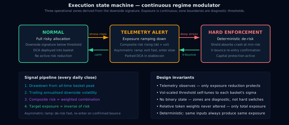
Normal → Telemetry Alert. When the drawdown signal or downside volatility signal rises above its respective threshold, the composite risk measure begins to increase. The target exposure drops below 100%. The exposure ramp begins reducing risk, with hysteresis between the de-risk and re-entry directions so that ordinary chop does not generate round-trip trades. DCA is still deployed into the basket but the system is no longer fully invested.
Telemetry Alert → Hard Enforcement. When target exposure drops below the redeploy threshold, the system enters full defensive mode. Parked DCA accumulates in stablecoin. The shield is absorbing the crash at deterministically reduced risk. This is the only zone where capital is actually being protected — telemetry alone does nothing.
Hard Enforcement → Normal. Recovery is not a binary switch. The adaptive engine tracks the trough since the last basket all-time high and accelerates re-entry when a confirmed V-bounce is detected — but only when the bounce impulse clears a confirmation threshold, protecting against dead-cat rallies. The ramp naturally tracks the basket recovery because drawdown shrinks as the equity curve heals.
The critical design property: telemetry never protects capital. The drawdown and volatility signals are inputs to a deterministic exposure function. The only thing that limits drawdown is the system's physical reduction of risky exposure. This is the difference between a risk dashboard and a risk controller.
4. The adaptive approach
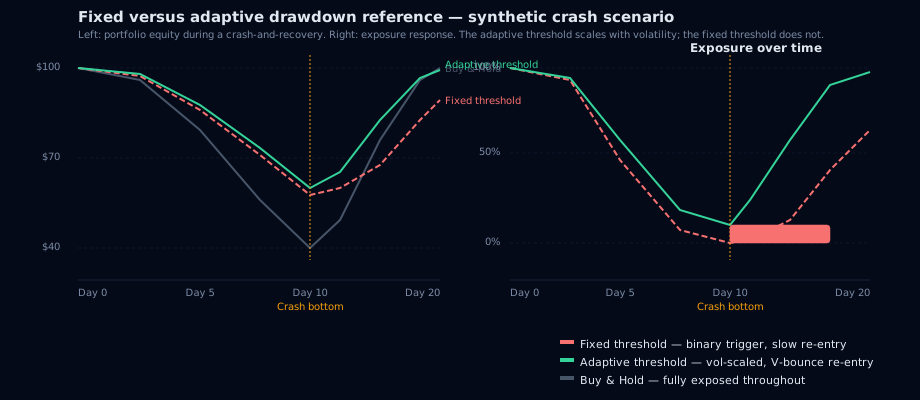
The adaptive threshold engine replaces the fixed drawdown reference with a volatility-scaled one. Instead of comparing the portfolio's drawdown to a constant level, the system measures the basket's own trailing annualised downside volatility and scales every threshold proportionally.
The effect is basket-relative sensitivity: a dip that is statistically ordinary for a low-volatility basket and a considerably larger dip that is statistically ordinary for a high-volatility basket produce the same response, because the reference moves with each basket's own realised risk instead of sitting at a fixed level. The scaling law and its multiplier are withheld. One engine, two sensitivity profiles, no manual tuning per basket type.
The difference between the two engines lies in threshold sensitivity and in how re-entry behaves once a bounce is confirmed. Ramp speeds and signal weightings are withheld for both.
5. Walk-forward head-to-head comparison
Both engines run on the identical production KKT-180 macro loop (risk-parity weights re-optimised every 180 days on trailing data), identical fee model (10 bps per trade, DCA buy and redeploy), identical DCA schedule. The only difference is the exposure-capping engine.
All metrics below are walk-forward out-of-sample. Each engine runs continuously on the rolling 180-day bounded window with cold replay and persisted shield state — the exact production data path. No in-sample full-window optimisation, no lookahead. The numbers represent what the system would have delivered in real time, not what looks best in hindsight.
Two baskets, selected for structural contrast:
| Majors | BTC, ETH, BNB, SOL, XRP, ADA, PAXG — seven tokens, low-volatility core with a gold anchor |
| Alts | XMR, BCH, XLM, LINK, CEL, QNT, HBAR, PAXG — eight tokens, structurally larger daily moves. CEL is a deliberate dead-token stress (Celsius, collapsed 2022); the ADV-K2 liveness screen zero-weights it once it fails the $1M/day trailing-volume test |
Settings: lump-sum start, 180-day optimizer warm-up, rolling 180-day bounded window, cold replay with persisted shield state, 2,095 measured intervals on majors and 2,316 on alts. Walk-forward OOS — no in-sample fitting.
5.1 Majors basket (walk-forward OOS)
| Metric | Fixed Threshold | Adaptive Threshold |
|---|---|---|
| Sharpe | 1.52 | 1.63 |
| Calmar | 1.82 | 2.00 |
| Max Drawdown | 25.7% | 23.1% |
| CAGR | 46.8% | 46.2% |
| Average exposure | 0.515 | 0.443 |
| Defensive days | 44.6% | 50.1% |
5.2 Alt basket (walk-forward OOS)
| Metric | Fixed Threshold | Adaptive Threshold |
|---|---|---|
| Sharpe | 1.03 | 1.10 |
| Calmar | 1.00 | 1.29 |
| Max Drawdown | 36.8% | 29.4% |
| CAGR | 36.7% | 37.9% |
| Average exposure | 0.4351 | 0.4349 |
| Defensive days | 56.9% | 46.5% |
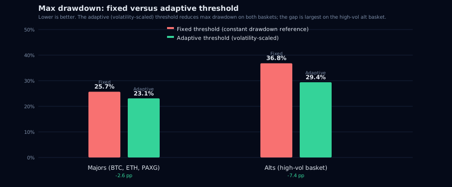
The adaptive engine wins on Sharpe, Calmar and max drawdown for both baskets. The largest gap is on the alt basket's max drawdown — 29.4% versus 36.8%, a 7.4 percentage-point reduction. That is the fixed-threshold failure mode in numbers: a reference level tuned for one volatility regime over-reacts on another.
The last two rows are the ones that decide whether that gap means anything, and they split the two baskets. On alts the engines hold identical average exposure (0.4349 versus 0.4351 — the same to four decimals), so the 7.4 pp drawdown gap is exposure-matched by construction and cannot be a level effect. On majors they do not: the adaptive engine holds 7.3 pp less exposure on average, so its drawdown advantage is not matched, and it has to be tested rather than asserted. Section 5.4 runs that test.
5.3 Reading
On the majors basket the improvement is meaningful but modest — the fixed threshold was already a reasonable fit for the volatility profile. On the alt basket the improvement is large — the fixed threshold was structurally mismatched, spending 56.9% of days in defense while still absorbing a 36.8% drawdown.
The adaptive engine's vol-scaled threshold automatically tunes itself to each basket. No separate configuration, no profile classification, no manual override.
5.4 The exposure-matched control — does the timing earn its keep?
A drawdown cut is not, on its own, evidence of skill. Any rule that holds less than full exposure on average will cut drawdown in almost every window, because the reduction can come from the level of exposure rather than from the timing of it. A claim of "the shield cut max drawdown by X pp" is untestable until it is compared against the dumbest possible alternative holding the same average risk.
So we ran that alternative. The constant-exposure control has no signal, no state, no thresholds and no memory: the identical KKT weight stream, scaled every day to a fixed fraction equal to the shield's own time-average exposure, on the identical production path. It pays no turnover fee, and as shown below it receives a further analytic advantage — the test is deliberately biased in the control's favour.
Majors basket
| Leg | Sharpe | Calmar | Max Drawdown | CAGR | Avg exposure | Fees |
|---|---|---|---|---|---|---|
| Buy & Hold | 1.37 | 1.23 | 55.9% | 68.7% | 1.000 | — |
| Fixed threshold | 1.52 | 1.82 | 25.7% | 46.8% | 0.515 | 0.021 |
| Adaptive threshold | 1.63 | 2.00 | 23.1% | 46.2% | 0.443 | 0.034 |
| Constant 0.515 (fixed engine's mean) | 1.23 | 1.06 | 32.5% | 34.5% | 0.515 | 0 |
| Constant 0.443 (adaptive engine's mean) | 1.19 | 1.04 | 28.4% | 29.5% | 0.443 | 0 |
Alts basket
| Leg | Sharpe | Calmar | Max Drawdown | CAGR | Avg exposure | Fees |
|---|---|---|---|---|---|---|
| Buy & Hold | 1.18 | 1.23 | 59.8% | 73.2% | 1.000 | — |
| Fixed threshold | 1.03 | 1.00 | 36.8% | 36.7% | 0.4351 | 0.028 |
| Adaptive threshold | 1.10 | 1.29 | 29.4% | 37.9% | 0.4349 | 0.039 |
| Constant 0.435 (both engines' mean) | 1.09 | 1.05 | 30.8% | 32.3% | 0.435 | 0 |
The two alts engines hold means that differ only in the fifth decimal, so their constant controls are near-identical but not bit-identical: 30.9% max drawdown at the fixed engine's mean (0.4351), 30.8% at the adaptive engine's (0.4349). The table shows the adaptive-matched leg; prose comparing the fixed engine to its own control uses 30.9%.
Four conclusions.
1. On majors the adaptive engine beats its own exposure-matched constant on every metric — Sharpe 1.63 versus 1.19, Calmar 2.00 versus 1.04, max drawdown 23.1% versus 28.4%, CAGR 46.2% versus 29.5% — while paying fees the control does not pay. The fixed engine also beats its own constant (Sharpe 1.52 versus 1.23, drawdown 25.7% versus 32.5%). On this basket the timing earns its keep, and the majors drawdown advantage in §5.1 is not a level effect.
2. On alts the fixed engine loses to a constant. A signal-free 0.435 exposure is shallower (30.9% versus 36.8%) and smoother (Sharpe 1.09 versus 1.03) than the fixed-threshold shield holding the same average exposure. That is §2.1's permanent-defense failure measured rather than asserted: an always-on shield is worse than simply being smaller, always. The adaptive engine wins the same comparison — drawdown 29.4% versus 30.8%, Calmar 1.29 versus 1.05 — but only ties on Sharpe (1.10 versus 1.09).
3. The return advantage is significant on majors and not on alts. A paired block bootstrap (1,000 resamples, 20-day blocks drawn jointly so the pairing survives) puts the adaptive engine's annualised log-growth advantage over its own constant at +11.7 pp on majors (90% interval +3.1 to +21.7) and +4.5 pp on alts (90% interval −4.2 to +14.4). The majors advantage clears zero; the alts advantage does not. Against the fixed engine's constant, the fixed engine itself scores +8.4 pp on majors (interval −0.7 to +18.2) and +3.9 pp on alts (interval −5.6 to +14.2).
4. The control's own handicap is measured, not assumed. Matching the mean of a time-varying exposure does not match its variance, and the difference is not neutral: under standard log-growth arithmetic a constant leg receives a variance-related growth allowance for free that a time-varying leg with the same mean does not. We evaluated that allowance on the realised exposure path (dispersion 0.245 majors / 0.223 alts) rather than assuming it away. It runs in the control's favour, at +0.65 pp/yr on majors and +0.83 pp/yr on alts — small against the gaps above, but it belongs on the record, and it is why a mean-matched constant is a strong control rather than a strawman: the shield's advantage is measured after granting the control that head start. The closed-form expression is withheld along with the rest of the engine's mathematics.
Where the control wins. Max drawdown is an extremum statistic: its effective sample size is the number of independent crash episodes (five or six across 6.5 years), not the 2,095 daily observations. Sliced per regime, the adaptive engine is shallower than its own constant in 3 of 5 regimes on majors and 3 of 6 on alts.
| Regime | Majors — adaptive | Majors — constant | Alts — adaptive | Alts — constant |
|---|---|---|---|---|
| Mar-2020 crash | not in window | not in window | 2.9% | 3.2% |
| May-2021 unwind | 20.5% | 16.4% | 20.6% | 14.2% |
| LUNA contagion | 11.3% | 22.2% | 9.9% | 20.6% |
| FTX collapse | 8.1% | 10.7% | 15.6% | 10.6% |
| Aug-2024 carry unwind | 10.5% | 6.4% | 8.9% | 13.4% |
| 2025-26 corrections | 15.5% | 20.3% | 21.3% | 17.5% |
The majors measurement window opens after the March-2020 crash, which is why that regime has five rows on one basket and six on the other.
The full-window advantage is concentrated in the deepest regimes — LUNA-class contagion and the 2025-26 correction on majors, LUNA and Aug-2024 on alts. In short, fast regimes the constant is equal or better. Anyone reading the 23.1% headline as "the shield wins every crash" is reading too much into it. The defensible claim is narrower and stronger: the shield wins the crashes that actually set the full-window maximum, and it beats a signal-free constant of the same average size on risk-adjusted return over the whole path.
5.5 Where the exposure minimum sits
A volatility-scaled rule has a known failure mode. Realised volatility rises after the drop and falls after the bounce, so the rule reaches its smallest exposure near the bottom — exactly when it should be re-entering. If the ramp in addition de-risks faster than it re-enters, that makes the problem worse on V-shaped recoveries, and V-shaped is most of what crypto does.
The adaptive engine is designed against this: once a bounce clears a confirmation threshold measured off the trough, its re-entry speed accelerates sharply and an exposure floor is unlocked, so that a genuine V is not sat out at minimum size. But a design intention is not a measurement, so we measured it. For every named regime and every defensive episode: the date of the basket's cumulative low versus the date of the shield's exposure low. Positive lag = exposure bottomed after price = the failure mode. Negative lag = the shield was already light going into the trough.
| Regime | Majors lag | Exposure at the basket low | Alts lag | Exposure at the basket low |
|---|---|---|---|---|
| Mar-2020 crash | not in window | — | +2 d | 0.20 |
| May-2021 unwind | −57 d | 0.41 | −56 d | 0.40 |
| LUNA contagion | −36 d | 0.15 | −32 d | 0.17 |
| FTX collapse | −40 d | 0.28 | −38 d | 0.30 |
| Aug-2024 carry unwind | +8 d | 0.61 | +36 d | 0.19 |
| 2025-26 corrections | +305 d | 0.26 | +312 d | 0.17 |
The failure mode is absent from the three deep crashes that define the full-window maximum. In May-2021, LUNA and FTX the shield's exposure bottomed 32–57 days before the basket did, at 0.15–0.41 exposure. It was light going in, not light at the bottom.
It is present in the fast, V-shaped ones. August-2024 is a four-week down-and-up move, and the shield's exposure minimum lands 8 days (majors) and 36 days (alts) after the basket's low. That is the same regime where the constant control beats the shield in §5.4 — the two findings corroborate each other instead of competing.
The 2025-26 lag (+305/+312 days) is not a missed bounce. That regime window is open-ended and the shield is still inside a live defensive episode at the time of writing, so its exposure minimum is recent by construction. The number measures "still defending," not "re-entered late."
Across all defensive episodes (18 on majors, 30 on alts) the median lag is +26 days and +54 days, with 67% and 70% of episodes bottoming after the basket. Read honestly: in short chop the shield systematically reaches its lowest exposure after the local low. That is a real cost. It is concentrated in episodes too small to move the full-window maximum, and it is the strongest argument in this study for the confirmed-bounce accelerator — which is also the part of the engine that short chop defeats, because a chop bounce never clears the confirmation threshold.
6. Per-profile empirical stress-test results — Aegis (v14) baseline
Attribution, corrected. Sections 6.1–6.4 report the Aegis (v14) fixed-threshold engine, not the Proteus (v18) adaptive engine compared in §5. They come from the walk-forward E2E harness running the frozen production default_config (the regime autopsy and the v14 unseen-token study) and they predate the adaptive engine's production wiring. An earlier revision of this page presented them as adaptive-engine results. That was incorrect and is corrected here.
They are retained because they stress-test the deleverage concept itself — a deterministic exposure dial on a KKT weight stream, telemetry never protecting capital — across named crash regimes, a dead token and unseen assets, and because they remain the largest body of published evidence in this project. They are not evidence about volatility-scaled thresholds, and nothing in §6 should be read as support for the adaptive engine specifically.
Every regime below was scored by parameters frozen before it happened — by construction out of sample.
6.1 Profile 1 — Majors + Gold (BTC, ETH, XRP, XMR + PAXG)
Low-volatility core with a gold anchor. Note this is a different basket from the §5 majors profile — four tokens plus the gold anchor, on a different data source and window. The two are not interchangeable.
| Regime | Window | Shield MDD | B&H MDD | Cut |
|---|---|---|---|---|
| R2 May-2021 unwind | 2021-04 → 2021-07 | 15.9% | 23.9% | +8.0 pp |
| R3 LUNA contagion | 2022-04 → 2022-06 | 16.8% | 44.1% | +27.3 pp |
| R4 FTX collapse | 2022-10 → 2023-01 | 3.3% | 13.3% | +9.9 pp |
| R5 Aug-2024 carry unwind | 2024-07 → 2024-09 | 12.4% | 17.5% | +5.0 pp |
| R6 2025-26 corrections | 2025-01 → 2026-08 | 18.9% | 32.1% | +13.2 pp |
Full-window (2020-03 → 2026-08, 2,327 days): Calmar 0.57 vs 0.38 B&H. MaxDD 16.9% vs 43.2% B&H. The shield gives up $7,414 of final equity ($15,650 vs $23,064 B&H) but delivers 50% more risk-adjusted efficiency per unit of drawdown risk.
6.2 Profile 2 — 2019-20 Generation (ETH, LINK, ATOM, DOT + PAXG)
Higher-volatility basket from the last cycle generation. The fixed drawdown reference is a poor fit here, and the per-regime cuts below are the concept working despite that mismatch rather than because of any self-tuning.
| Regime | Window | Shield MDD | B&H MDD | Cut |
|---|---|---|---|---|
| R2 May-2021 unwind | 2021-04 → 2021-07 | 19.1% | 40.8% | +21.7 pp |
| R3 LUNA contagion | 2022-04 → 2022-06 | 21.3% | 44.8% | +23.5 pp |
| R4 FTX collapse | 2022-10 → 2023-01 | 1.9% | 9.2% | +7.3 pp |
| R5 Aug-2024 carry unwind | 2024-07 → 2024-09 | 9.5% | 15.0% | +5.5 pp |
| R6 2025-26 corrections | 2025-01 → 2026-08 | 22.5% | 34.9% | +12.4 pp |
Full-window (2021-02 → 2026-08, 1,998 days): MaxDD 18.9% vs 37.5% B&H — the shield halved the drawdown. Per-regime cuts are uniformly positive. The full-window Calmar favours B&H (0.12 vs 0.19) — this is the honest limit of the claim: per-regime protection yes, but on this specific basket the bull legs were large enough that the protection cost more in participation than it saved in drawdown.
6.3 Profile 2 stress — Landmine basket (BTC, ETH, CEL + PAXG)
Deliberately includes a token that went to zero (Celsius). The Aegis (v14) shield ran with the ADV-K2 liveness screen active, which zeroed CEL's weight once it failed the $1M/day trailing-volume test.
| Regime | Window | Shield MDD | B&H MDD | Cut |
|---|---|---|---|---|
| R3 LUNA contagion | 2022-04 → 2022-06 | 4.1% | 11.4% | +7.3 pp |
| R4 FTX collapse | 2022-10 → 2023-01 | 5.4% | 17.8% | +12.4 pp |
| R5 Aug-2024 carry unwind | 2024-07 → 2024-09 | 9.8% | 11.8% | +1.9 pp |
| R6 2025-26 corrections | 2025-01 → 2026-08 | 20.1% | 32.9% | +12.8 pp |
Full-window Calmar 0.65 vs 0.50 B&H — the best risk-adjusted efficiency of all three baskets. The dead token stress confirms: the shield + liveness screen handles catastrophic individual-asset failure without manual intervention.
6.4 OOS validation — 16 unseen token baskets, and what "16" actually means
An out-of-sample test on baskets of tokens never used to design or tune the system. The 16 are all k=3, k=4 and k=5 combinations of five survivors — AVAX, CRO, DOGE, HBAR, LINK — which is 10 + 5 + 1. PYTH (short history, launched 2023-11) and CEL (dead token) are separate stress cases outside the 16, not members of it.
| Metric | Result |
|---|---|
| Max-drawdown reduction | median +54.3 pp (min +46.7, max +65.8) — reduced DD in 16 / 16 baskets |
| Calmar delta | median +0.35 — improved in 16 / 16 |
| Sharpe delta | median +0.16 — improved in 15 / 16 |
What this establishes, and what it does not. The 16 are not 16 independent trials. Every one is a subset of the same five assets over the same three date windows (2,118 / 2,489 / 2,764 bars), so a single 2022-shaped drawdown moves all sixteen simultaneously. A sign test over sixteen draws this correlated has an effective sample size closer to one regime than to sixteen. The honest description is five unseen assets observed through one market history, and the +54.3 pp median is one large measurement, not sixteen confirmations.
The benchmark compounds the problem. Buy & Hold in that study is 100% exposed while the modulator's average exposure is far below 1, so a drawdown reduction is close to guaranteed before any signal is evaluated. Section 5.4 is the experiment that removes that guarantee — it re-runs the comparison against a constant sized to the shield's own average exposure — and §6.4 should be read against it, not instead of it.
The selection-bias correction this count deserves is applied elsewhere in the corpus: the Monte Carlo & selection-bias study computes deflated Sharpe ratios against the number of configurations actually tried in this project's history. It was not applied here. That is an omission, not a disagreement.
What survives the correction is narrower and still real: no parameter of the engine was tuned on any of these five assets, and the drawdown-reduction mandate held on every subset including the dead-token stress.
6.5 Execution robustness
A robustness study of 129 walk-forward re-runs — perturbing every user-facing knob one at a time, stress-testing fees to 20× and execution to 2 days late — found no cliff:
| Stress | MaxDD degradation | Sharpe degradation |
|---|---|---|
| DCA delay (2-5 days) | −0.1 pp | −0.003 |
| DCA amount ±20% | +0.0 pp | +0.001 |
| Skip every 4th DCA | +0.5 pp | +0.051 |
| Fee × 20 | < 2 pp | < 0.10 |
| Execution 2 days late | < 3 pp | < 0.08 |
The drawdown cut survives late execution almost intact on the perturbation harness. The shield's threshold rebalancing (only trade when the target drifts beyond the deadband) naturally reduces fee drag — approximately 64% fewer rebalances versus continuous adjustment.
One published study disagrees on magnitude. The Human Factor / execution-error study found that on the production KKT stack a 3-day execution lag adds +4.7 to +11.3 pp of drawdown and fails its protection gates, because the ramp on the production portfolio is gentler than on the equal-weight test basket. Both results are correct on their own harness; the perturbation table above is the optimistic bound and the execution-error study is the pessimistic one. Neither should be quoted alone.
See the Regime Autopsy study for the full per-regime decomposition, the OOS Validation study for per-basket detail, and the Static vs Dynamic study for the comparison against 60/40, 70/30, and 80/20 static allocations. Those three static splits all sit above the shield's realised average exposure (0.44 majors / 0.43 alts), which is why the exposure-matched control in §5.4 was necessary rather than redundant.
7. Caveats
- A drawdown cut is not, by itself, evidence of skill. Any rule holding less than full exposure on average cuts drawdown in most windows. Every protection claim on this page is reported next to a constant-exposure control matched to the claiming engine's own average (§5.4), and where the control wins, the page says so.
- Max drawdown is an extremum statistic. Its effective sample size is the number of independent crash episodes — five or six across 6.5 years — not the 2,000+ daily observations. Full-window drawdown figures are single-episode outcomes. Per-regime, the adaptive engine beats its own matched constant in only 3 of 5 regimes on majors and 3 of 6 on alts.
- The shield does not beat buy-and-hold on risk-adjusted return on the alt basket. B&H scores Sharpe 1.18 there against the adaptive engine's 1.10; the shield wins on Calmar (1.29 vs 1.23) and max drawdown (29.4% vs 59.8%) and loses on CAGR (37.9% vs 73.2%). On majors the shield wins Sharpe too (1.63 vs 1.37). Claims of "wins on every metric" apply only to the fixed-versus-adaptive pairing, never to the buy-and-hold comparison.
- Absolute return trade-off. The adaptive engine, like any defensive system, gives up final equity versus buy-and-hold in windows that contain strong bull legs. In every full-window comparison the protective system trails buy-and-hold on raw final value. The improvement is in risk-adjusted efficiency (Calmar, Sharpe) and max drawdown.
- Warm-up period. The trailing-volatility measurement needs a minimum window to stabilise. Below that minimum history the dispatcher falls back to the fixed-threshold engine rather than emit an under-warmed reading; during warm-up the system uses a conservative floor threshold. This is the graceful-degradation path, not the tuned behaviour.
- The adaptive threshold is still self-referential. It scales with the basket's own trailing volatility, so it is a function of the data it is applied to. It survives the bounded production window because the trailing statistic is window-local and clamped to an absolute band rather than expanding — which is exactly what killed the expanding-percentile engine in §2.2 — but it belongs on the same permanent watch-list, and it must be re-tested if the window length ever changes.
- Same-day open gaps are uncatchable. Any daily-close system can only react to what happens between closes. Crypto crashes are drift-dominated (95–100% of damage unfolds in the intraday leg), but the uncatchable residual concentrates in single worst days.
- Simulated results. Every figure in this study is computed from historical price data by a backtest. No capital was invested and no orders were placed. Figures exclude slippage and liquidity effects, though a simulated 0.1% exchange fee is charged on every trade. Parked stablecoin earns zero in the harness, which penalises both shields equally and the constant control identically.
8. Methodology
1. MACRO loop: KKT risk-parity optimisation on the trailing 180-day window, re-run every 180 days; weights frozen in between. Both engines share the identical macro loop and receive the same weights. 2. DAILY loop: Each exposure-capping engine evaluated on every daily close. Threshold rebalancing only trades when the target drifts beyond the deadband; 10 bps fee on every trade, DCA buy and redeploy. 3. Validation path: Rolling 180-day bounded window, cold replay, persisted shield state — the exact data path the production system runs. Not a continuous backtest on all available history. All reported metrics are walk-forward out-of-sample. 4. Metrics: TWR daily returns (DCA flows removed), risk-free rate 5%; max drawdown from the virtual equity peak. 5. Engines compared: Aegis (v14) is the fixed-threshold baseline; it was the production engine when this study ran and now serves only as a warm-up fallback. Proteus (v18) is the adaptive engine and is the production engine today; it replaces the constant drawdown reference with one that scales with the basket's own trailing volatility, and it accelerates re-entry once a bounce is confirmed rather than waiting for the drawdown to shrink on its own. Every numeric setting of both engines is withheld — reference levels, the weighting between the drawdown and downside-volatility signals, ramp speeds and whether they are symmetric, scaling multipliers, clamp bands, warm-up floors and bounce-confirmation triggers — as is the closed-form arithmetic behind the variance handicap in §5.4. These are the tunable surface of the product: publishing the numbers together with the structure would make the rule replicable from this page alone. What is disclosed here is the class of mechanism, the measured behaviour, and the fact that neither engine was re-tuned for this comparison. Both are post-processors on the same KKT weight stream — relative token proportions are never altered, only total risky exposure changes. 6. Constant-exposure control: no signal, no state, no thresholds. The identical KKT weight stream scaled to a fixed fraction equal to each shield's own time-average exposure, on the same window and fee convention. The control pays no turnover fee. Exposure dispersion is measured on the daily exposure path so the control's analytic variance handicap — a log-growth allowance a mean-matched constant receives for free, quantified in §5.4 and whose closed form is withheld — can be discounted from its result. 7. Uncertainty: paired block bootstrap, 1,000 resamples of 20-day blocks drawn jointly on the paired daily returns so the pairing survives. Applied to the annualised log-growth gap, which is additive and therefore validly resampled. Deliberately not applied to max drawdown: reordering blocks destroys the exposure/crash alignment a state-dependent rule depends on, so a day-level bootstrap on a path-dependent extremum is a permutation robustness check, not a sampling interval. Drawdown uncertainty is reported per regime instead, where the independent unit is the crash episode. 8. Lag diagnostic: per named regime and per defensive episode, the index of the basket's cumulative low versus the index of the shield's exposure low, in days. Positive = exposure bottomed after price (the vol-targeting failure mode); negative = already light going in. 9. Data: Yahoo Finance daily closes (unadjusted) for the §6 regime stress tests; CoinGecko-derived daily closes for the §5 production path and the §6.4 OOS token validation. Common-date alignment per basket.
9. Verdict
- Fixed drawdown thresholds are basket-blind: a single number cannot serve both a low-volatility majors basket and a high-volatility altcoin basket. Measured, not asserted — on the alt basket a signal-free constant at the fixed engine's own average exposure is shallower (30.9% vs 36.8%) and smoother (Sharpe 1.09 vs 1.03) than the fixed shield itself.
- Full-history lookback truncation inverts the ranking on the production path when the winning signal needs more history than the production window supplies. This is not in-sample overfitting and walk-forward selection does not fix it (§2.2).
- The execution state machine separates telemetry (observation) from enforcement (deterministic exposure reduction). Only the latter protects capital.
- An adaptive threshold that scales with the basket's own trailing downside volatility solves both problems with a single engine — no per-basket tuning, no profile switching.
- On the production path the adaptive engine wins both baskets on Sharpe, Calmar and MaxDD against the fixed baseline. The alt-basket result is exposure-matched by construction (both engines average 0.435 exposure), so the 7.4 pp drawdown gap is a timing effect and not a level effect.
- The exposure-matched control confirms the timing earns its keep on majors and does not clearly do so on alts. Against a constant at its own average exposure the adaptive engine wins every metric on majors (Sharpe 1.63 vs 1.19, Calmar 2.00 vs 1.04, MaxDD 23.1% vs 28.4%, CAGR 46.2% vs 29.5%), with a bootstrap log-growth advantage of +11.7 pp/yr (90% interval +3.1 to +21.7). On alts it wins Calmar (1.29 vs 1.05) and ties Sharpe (1.10 vs 1.09), with a +4.5 pp/yr log-growth advantage whose interval spans zero (−4.2 to +14.4).
- The drawdown advantage is regime-concentrated. Per named regime the adaptive engine is shallower than its own matched constant in 3 of 5 regimes on majors and 3 of 6 on alts — winning the deep, slow contagion crashes and losing the short, fast ones. Max drawdown is an extremum statistic with an effective sample size of ~5 episodes, not 2,000 days.
- The vol-targeting failure mode is absent from the deep crashes and present in the fast ones. Exposure bottomed 32–57 days before the basket in May-2021, LUNA and FTX, and 8–36 days after it in the V-shaped Aug-2024 unwind. Across all defensive episodes the median lag is +26 days (majors) and +54 days (alts).
- Per-profile stress tests on the Aegis (v14) baseline: 15/15 regime-basket combinations show positive drawdown cuts versus buy-and-hold. Profile 1 (Majors+Gold) full-window Calmar 0.57 vs 0.38 B&H. Profile 2 (2019-20 Gen) MaxDD halved (18.9% vs 37.5%). These validate the deleverage concept, not the adaptive threshold (§6).
- 16 unseen-token baskets show improved Calmar in 16/16 and a median MaxDD reduction of 54.3 pp — but the 16 are overlapping subsets of the same five assets over the same windows, so the effective sample size is roughly one market regime, and the 100%-exposed benchmark makes a drawdown cut close to guaranteed a priori (§6.4).
- 15+ published studies exercise the approach across unseen tokens, named crash regimes, perturbed parameters and stressed fees. They are not independent confirmations of one another, and the two that disagree on execution-lag damage are both cited in §6.5.
Simulated results — no real money. Every figure is computed from historical price data by a backtest; no capital was invested and no orders were placed. Figures exclude slippage and liquidity effects, though a simulated 0.1% fee is charged on every trade. Simulated and past performance is not a reliable indicator of future results. AQMath is software, not investment advice.